Last Change: 2025-08-27 #dba #JT
 sphe_add_field_point
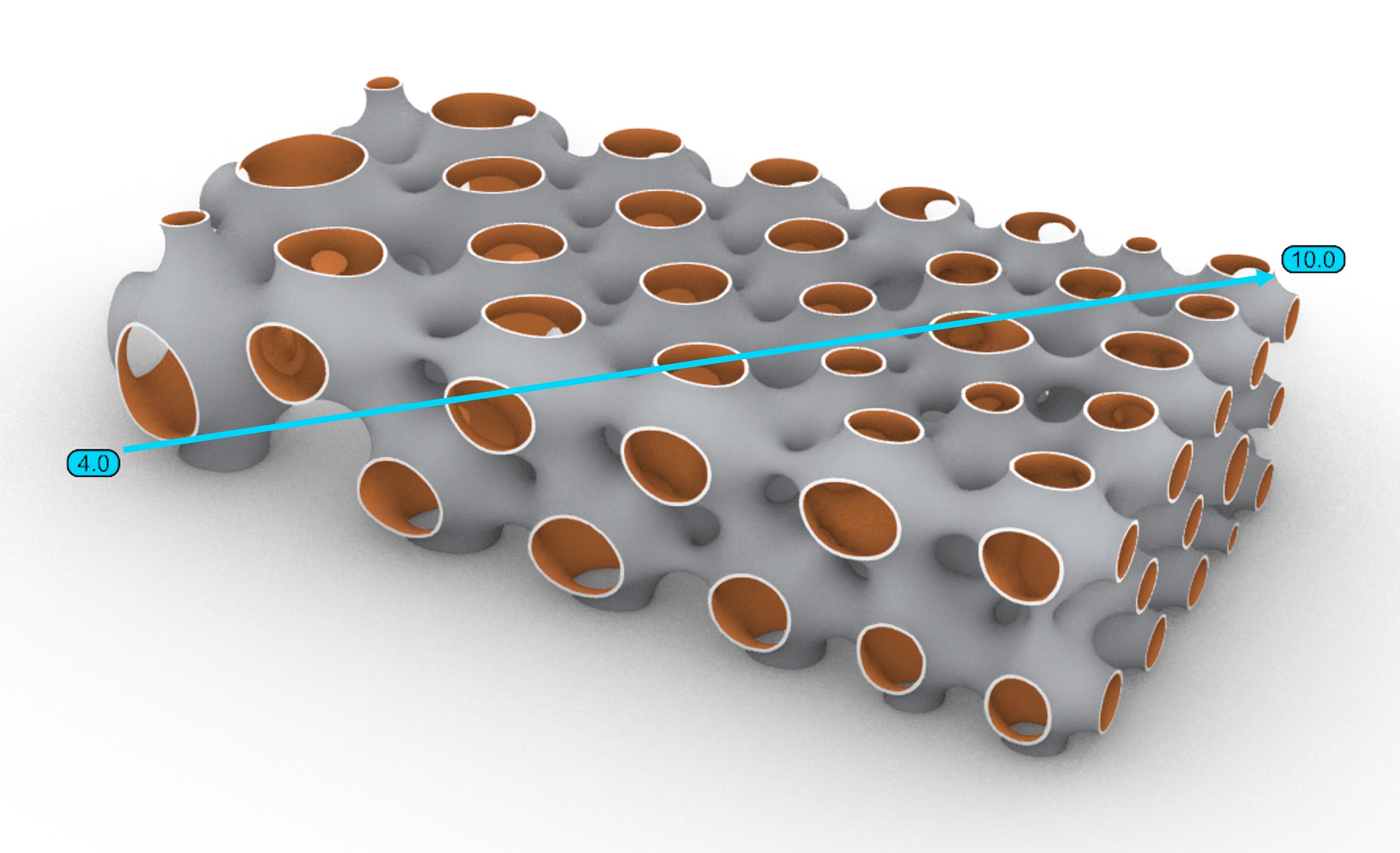
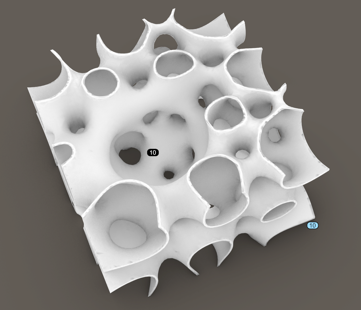
Using the sphe_add_field_point tool, you can modify any field parameter or create a field gradient. The figure below shows a generated Spherene structure with a density gradient along the diagonal.
Usage
Adds a Field Point to the project. A field is essentially a function that is calculated at a particular point in space.
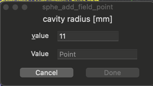
Double click a field point or edit its value using the spherene inspector :
Workflow
This video tutorial shows the workflow of how to use this tool (Made in older version, concept still applies to the current version).
The general steps include:
- Click the
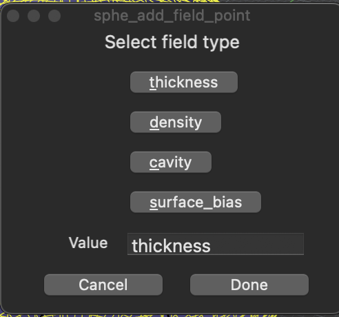
sphe_add_field_pointbutton. - In the pop-up window (for Mac users) or the command line (for Windows users), select the field parameter you want to modify and enter a new value.
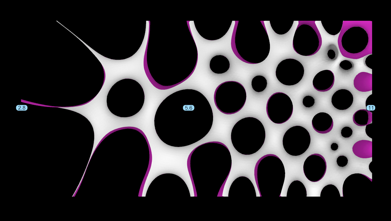
- Click on the point in the workspace where you want to apply the modification. You can repeat steps 1–3 to add additional points or modify more fields. The example below shows two modified points with different density values (indicated by blue text). This will create a density gradient along the diagonal.
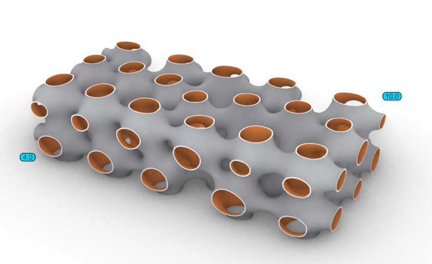
- Click the compute button
 , select Solid Surface, and start the computation. The example result is shown in the first figure.
You can download this example file here.
Parameters
- Type: Density, Thickness, Surface Bias, Cavity
- Value: Variable based on Type
- Position: Place and position point in 3D viewport
Density [%], Thickness [mm], Surface Bias [±1], Cavity [radius, mm]
Density
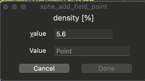
| Attribute | Value | Default | Unit |
|---|---|---|---|
| Color | Cyan | ||
| Range | 1 < | 5.6 | Volume Fraction |
Thickness
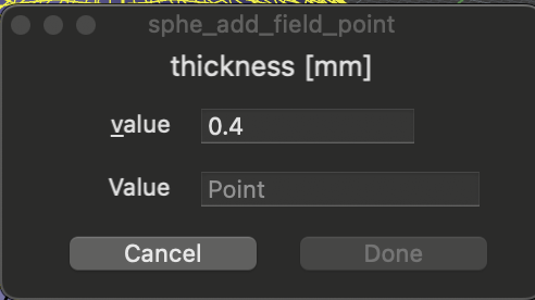
| Attribute | Value | Default | Unit |
|---|---|---|---|
| Color | Magenta | ||
| Range | 0.1 < | 0.4 | mm |
As long as you do not have a thickness field point set, the DRT acts as wall thickness by default. You can set the DRT in the compute dialogue.
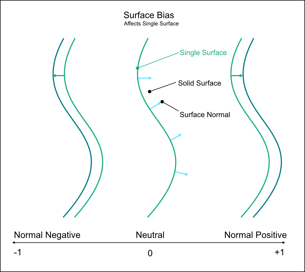
Surface Bias
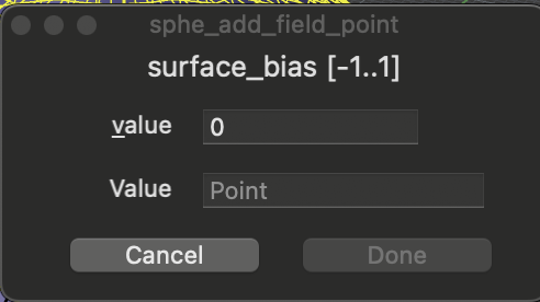
| Attribute | Value | Default |
|---|---|---|
| Color | Yellow | |
| Range | -1 to 1 | 0 |
Shifts the Single Surface, minimal surface, from its ideal position to the negative or positive of its normal.
Cavity
| Attribute | Value | Default | Unit |
|---|---|---|---|
| Value (radius) | 0 < | 11 | mm |
Adding a field point Cavity will create a spherical cavity. For more complex geometries, use the sphe_add_cavity tool.
Scatter Vector 1
| Attribute | Value | Default | Unit |
|---|---|---|---|
| X, Y, Z | non-zero vector | (0,0,1) | |
| W | 0 ≤ | 0 | mm |
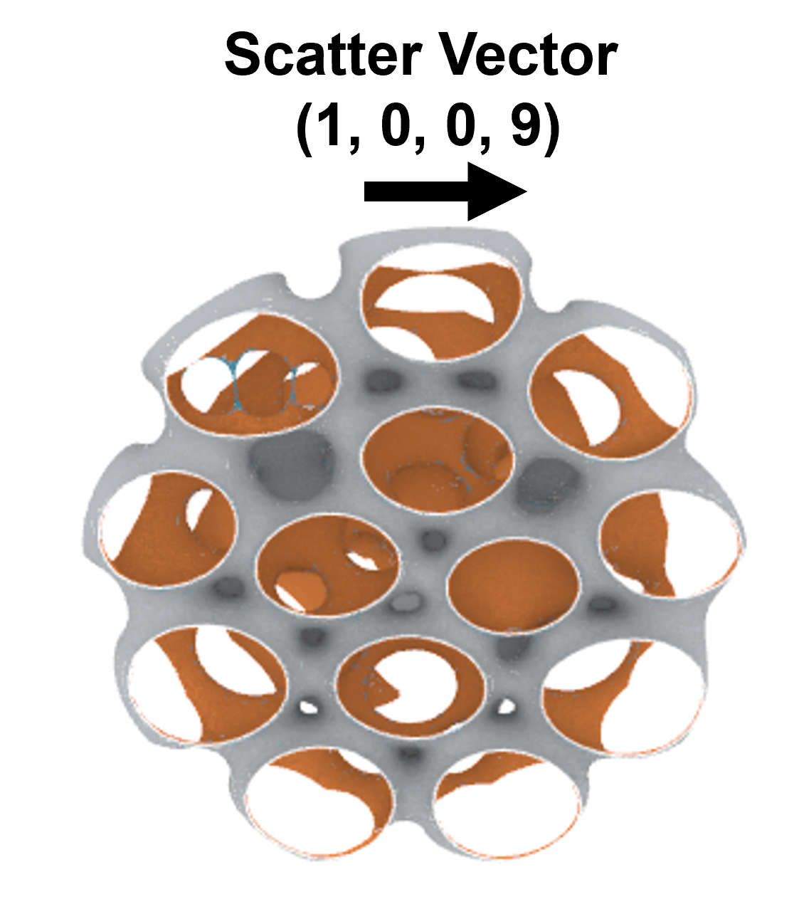
The introduction of scatter vectors controls the local stretching of the ADMS or flow ADMS. The (X, Y, Z) components are normalized and define the direction of the scatter vector. W defines the magnitude of the scatter vector, measured in millimeters.
Scatter Vector 2
| Attribute | Value | Default | Unit |
|---|---|---|---|
| X, Y, Z | non-zero vector | (0,0,1) | |
| W | 0 ≤ | 0 | mm |
Scatter Vector 2 has the same function as Scatter Vector 1. When combined with Scatter Vector 1, it allows the geometry to be stretched in two different directions with different magnitudes at each point.
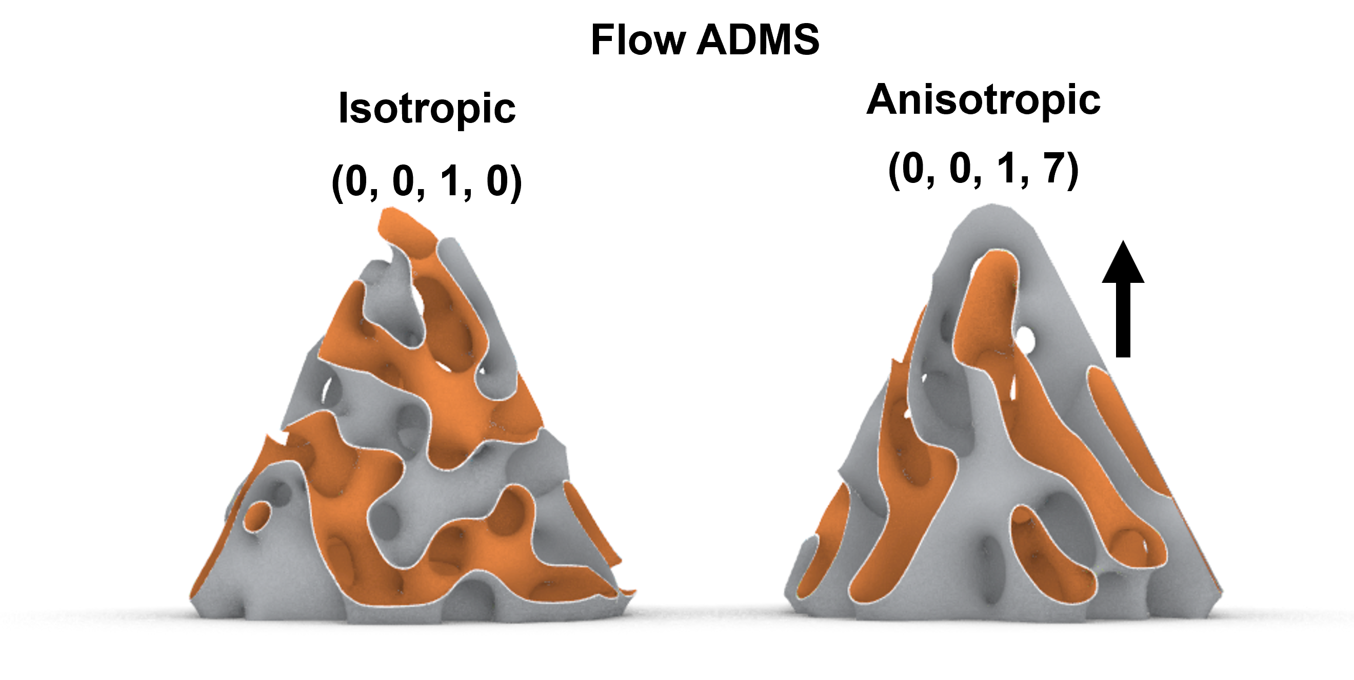
Flow Direction
| Attribute | Value | Default | Unit |
|---|---|---|---|
| X, Y, Z | non-zero vector | (0,0,1) | |
| W | 0 ≤ | 0 | 10% |
When a flow direction is defined, a Flow ADMS is generated. The (X, Y, Z) components are normalized and define the direction of flow. W defines the magnitude of the flow direction. When W=0, an isotropic Flow ADMS is generated. Otherwise, a directional preference following the (X, Y, Z) direction is applied. For example, W=7 indicates that 70% of the Flow ADMS surface tends to follow the (X, Y, Z) direction.
Examples
Density Field: Controlling the density:
Thickness Field: Controlling the wall thickness:

Cavity: Adds a cavity (Value is a radius) at the point location to push the minimal surface away:
Scatter Vector 1 & 2: Adds a vector at the point location to stretch the geometries:
Flow Direction: generate flow ADMS with and without directional preference: